Tree - Swim in Rising Water
All diagrams presented herein are original creations, meticulously designed to enhance comprehension and recall. Crafting these aids required considerable effort, and I kindly request attribution if this content is reused elsewhere.
Difficulty : Easy
Dijkstra’s Algorithm
Problem
You are given an n x n integer matrix grid where each value grid[i][j] represents the elevation at that point (i, j).
The rain starts to fall. At time t, the depth of the water everywhere is t. You can swim from a square to another 4-directionally adjacent square if and only if the elevation of both squares individually are at most t. You can swim infinite distances in zero time. Of course, you must stay within the boundaries of the grid during your swim. Return the least time until you can reach the bottom right square (n - 1, n - 1) if you start at the top left square (0, 0).
Example 1:
1
2
3
4
5
6
7
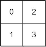
Input: grid = [[0,2],[1,3]]
Output: 3
Explanation:
At time 0, you are in grid location (0, 0).
You cannot go anywhere else because 4-directionally adjacent neighbors have a higher elevation than t = 0.
You cannot reach point (1, 1) until time 3.
When the depth of water is 3, we can swim anywhere inside the grid.
Example 2:
1
2
3
4
Input: grid = [[0,1,2,3,4],[24,23,22,21,5],[12,13,14,15,16],[11,17,18,19,20],[10,9,8,7,6]]
Output: 16
Explanation: The final route is shown.
We need to wait until time 16 so that (0, 0) and (4, 4) are connected.
Solution
Even though this problem is set as Hard, in LeetCode, it.s actually a fairly easy problem to solve. The hardest part is to understand the problem and not really the solution to it. In nutshell, we need find the shortest path from [0,0] to [N-1,N-1] with lowest max cost. Say we have two paths [1,1,5,1,1,1] and [2,3,2,2,3,2] the 2nd one is the answer as the max value is 3 than the max value of 5 in the first example.
Whenever we think about shortest path algorithm we first consider Dijkstra’s Algorithm.
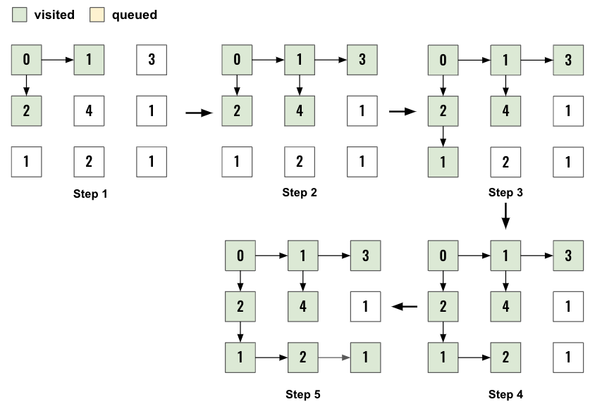
Let’s start with a better visualization. Here is a simpler problem to look at. We will be using a min_heap to find the shortest path.
So at every node, traverse using BFS and find the max cost then push the node to the min_heap. Then we pop the min from the mean_heap and traverse its neighbors. If at any point we reach node [N-1,N-1] we return the path cost. Below is the flow of the min_heap for the example above.
Main Difference to Dijkstra’s Algorithm
The code is almost exactly same as Dijkstra’s Algorithm. You can refer the explanation of that here if needed. However there are two places the implementations are different.
Cost/Time calculation:
- The calculation of cost/time to reach a node is different. In original Dijkstra’s Algorithm, we are just adding the cost/time for every traversal.
heapq.heappush(min_heap, (parent_weight+child_weight, child_node))
- However here we need to find the
maxcost/time between current node and the neighboring node we are planning to traverse as we can freely travel if the current elevation/cost/time is less thanmaxvalue in the current path.heapq.heappush(min_heap, (max(parent_cost, child_node_cost),r,c))
- The calculation of cost/time to reach a node is different. In original Dijkstra’s Algorithm, we are just adding the cost/time for every traversal.
Weight/Cost/Time impact on visited
There is another major difference between this algorithm implementation and default Dijkstra’s Algorithm’s implementation.Let me try to explain.
In default Dijkstra’s Algorithm, the weight/cost/time to reach a node is in the edge connecting two nodes. Now a node can be reached using various edges and each can have a different weight/cost/time. So it’s important to add the node multiple times (as many times as it has incoming edges) into the
min_heap.Here is an example,
3can be reached from either2or1.flowchart LR 1-->|1|2 2-->|2|3 1-->|4|3However, in the current problem does not matter how an edge can be reached the weight/cost/time is always fixed by its own value. So we shall not try to push the node into the
min_heapmore than once as this will cause themin_heapto overflow and timeout.For an example, the
4in the example outlined above, can be reached from 2 of its neighbors. Lets explore this step by step. There are two ways to solve this.Option 1: Add to
visitedset right after (or before) the node is pushed to themin_heap.Option 2: Follow the code structure as Dijkstra’s Algorithm, and skip processing if the node is already visited, however only after popping the node from the
min_heap. This way themin_heapwon’t grow larger.
So in nutshell, there are two ways to solve this problem however same is not true for the Dijkstra’s Algorithm.
Let’s explore Option 2 first as the code is more similar to Dijkstra’s Algorithm.
Define all the variables needed.
1
2
3
4
5
6
N=len(grid)
cost_at_start = grid[0][0]
min_heap = [[cost_at_start,0,0]]
directions=[[0,1],[1,0],[-1,0],[0,-1]]

visited=set()
Start the while loop and pop the node from min_heap
1
2
while min_heap:
  t, r, c = heapq.heappop(min_heap)
In case the last node is reached, return the weight/time/cost.
1
2
  if r == N-1 and c == N-1:
    return t
If the node is already visited, skip rest of the processing do not traverse its neighbors.
1
2
  if (r,c) in visited:
    continue
Otherwise, add the node to the visited.
1
  visited.add((r,c))
Now, just like in default Dijkstra’s Algorithm push all its neighbors only if it’s not out of bound and not visited. The other difference as we saw earlier is the max weight based on the node value.
1
2
3
4
5
6
  for dr,dc in directions:
    nei_r= r+dr
    nei_c= c+dc
    if nei_r < 0 or nei_c <0 or nei_r==N or nei_c==N or (nei_r,nei_c) in visited:
      continue
    heapq.heappush(min_heap, (max(t, grid[nei_r][nei_c]),nei_r,nei_c))
Let’s explore the Option 1. All the variable initialization are same as before.
1
2
3
4
5
N=len(grid)
cost_at_start = grid[0][0]
min_heap = [[cost_at_start,0,0]]
directions=[[0,1],[1,0],[-1,0],[0,-1]]
visited=set()
The only difference is we are going to add the starting node into the visited set.
1
visited.add((0,0))
Now remaining part is same as well.
1
2
3
4
5
while min_heap:
  t, r, c =heapq.heappop(min_heap)

  if r == N-1 and c == N-1:
    return t
We won’t have to verify or add the node to the visited set as the node will already be inside visited set. We can directly add it’s neighbors to the min_heap. (Same code as Option 2)
1
2
3
4
5
6
  for dr,dc in directions:
    nei_r= r+dr
    nei_c= c+dc
    if nei_r < 0 or nei_c <0 or nei_r==N or nei_c==N or (nei_r,nei_c) in visited:
      continue
    heapq.heappush(min_heap, (max(t, grid[nei_r][nei_c]),nei_r,nei_c))
Now, once the node is added to the min_heap, add it to visited as well.
1
visited.add((nei_r,nei_c))
Here are the two flow charts.
Final Code
Here is the full code.
Option 1:
1
2
3
4
5
6
7
8
9
10
11
12
13
14
15
16
17
18
19
20
def swin_in_water(grid):
    N = len(grid)
    directions = [[1, 0], [0, 1], [-1, 0], [0, -1]]
    min_heap = [[grid[0][0], 0, 0]]
    visited = set((0, 0))

    while min_heap:
        t, r, c = heapq.heappop(min_heap)

        if r == N-1 and c == N-1:
            return t

        for dr, dc in directions:
            nei_r = r+dr
            nei_c = c+dc
            if nei_r < 0 or nei_c < 0 or nei_r == N or nei_c == N or (nei_r, nei_c) in visited:
                continue
            heapq.heappush(
                min_heap, (max(t, grid[nei_r][nei_c]), nei_r, nei_c))
            visited.add((nei_r, nei_c))
Option 2:
1
2
3
4
5
6
7
8
9
10
11
12
13
14
15
16
17
18
19
20
21
22
23
24
25
26
def swin_in_water(grid):
    N = len(grid)
    directions = [[1, 0], [0, 1], [-1, 0], [0, -1]]
    min_heap = [[grid[0][0], 0, 0]]
    visited = set()

    while min_heap:
        t, r, c = heapq.heappop(min_heap)

        if r == N-1 and c == N-1:
            return t

      	if (r, c) in visited:
          continue

       	visited.add((r,c))

        for dr, dc in directions:
            nei_r = r+dr
            nei_c = c+dc
            if nei_r < 0 or nei_c < 0 or nei_r == N or nei_c == N or (nei_r, nei_c) in visited:
                continue
            heapq.heappush(
                min_heap, (max(t, grid[nei_r][nei_c]), nei_r, nei_c))


